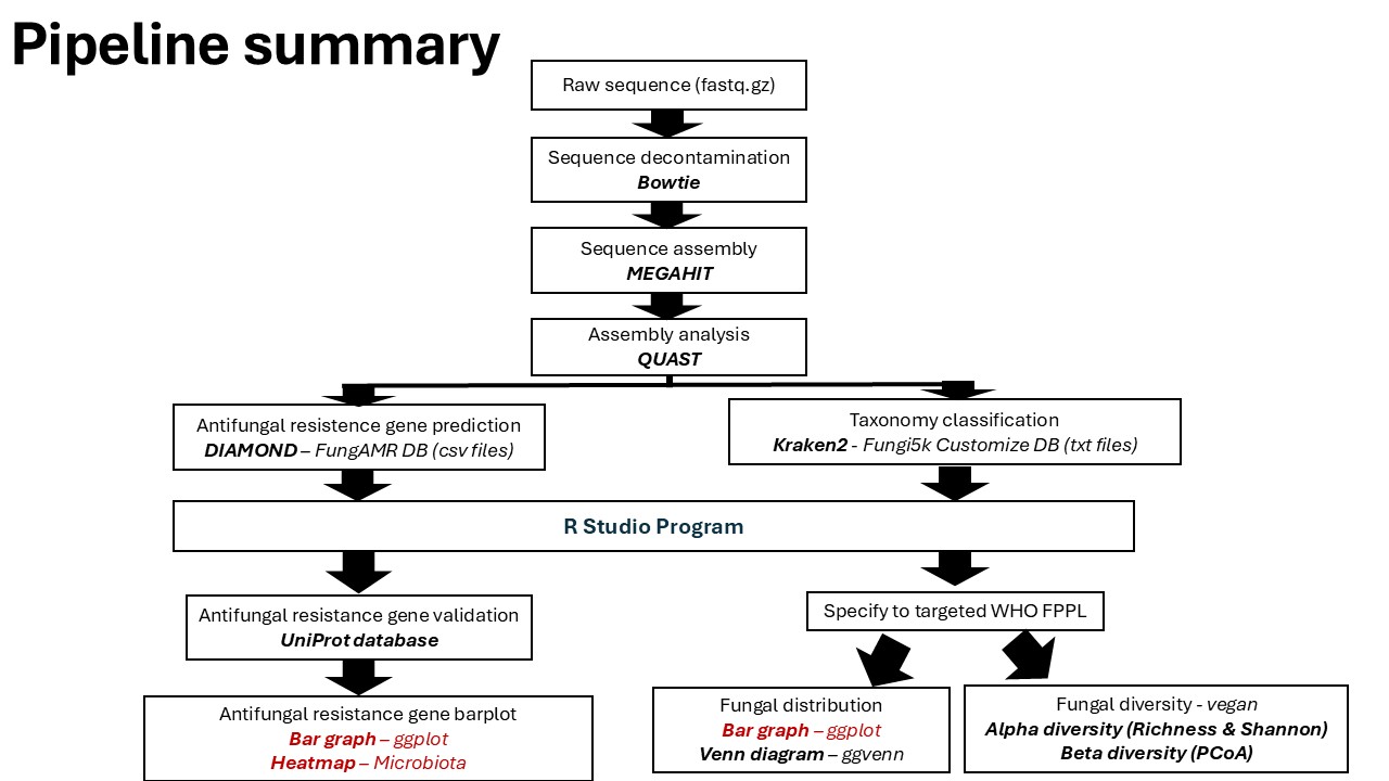
Metagenomics post processing (Data visualization and analysis)
Metagenomics post-processing refers to the set of analytical and interpretative steps applied after raw sequencing data have been quality-controlled, assembled, and taxonomically or functionally profiled. This stage focuses on transforming complex metagenomic outputs into biologically meaningful insights through data visualization, statistical analysis, and integrative interpretation.

This tutorial combines the workflows for analyzing WHO Fungal Priority Pathogens (WHO FPPL) and Antimicrobial Resistance (AMR) Genes into a single, cohesive guide. It assumes you have already processed your raw reads into count tables (as covered in the previous data processing step).
Glimpse of R program & R studio
R program is a free, open-source integrated development environment (IDE) for the R programming language, widely used for data analysis, visualization, and statistical interpretation.
Install R
Install Rstudio
Tutorial for basic R in ecology
Please check our video tutorial WHO FPPL visualization ▶️here and downloading our training data 📁here.
Additional information for R color palette here and ggplot info1 / info2.
Fungal Metagenomics Data Visualization Pipeline
Step 0: Open Rstudio cloud and Launch Console

Once you log in to Rstudio cloud, your web browser should bring up a similar window as the picture shown above. Click the button on the top right corner to create a new Rstudio project. Then, the next step is to click “Terminal” which should look like a picture below after you click on it.
R script: T1_MGS data processing_HPCC.Rmd
Prerequisites Ensure you have the following R packages installed and loaded. These libraries are essential.
library(tidyr)
library(tidyverse)
library(stringr)
library(readr)
library(dplyr)
Step 1: Data preparation
Put all txt file of kraken result into one folder Adjust the folder & pattern to your files (e.g., RK1.txt, RB1.txt, …)
## 1. Path to folder containing all report files
folder <- "C:/Users/ASUS/Downloads/TrainingFAILSAFE/Training data/sequence"

## 2. List all txt files in that folder

files <- list.files(folder, pattern = "\\.txt$", full.names = TRUE)
## 3. Derive sample IDs from file names (strip path and extension)
sample_ids <- tools::file_path_sans_ext(basename(files))
# 4. Function to read one kraken report (all ranks)
read_kraken_report <- function(file, sid){
  df <- read.table(file,
                   sep = "\t",
                   header = FALSE,
                   quote = "",
                   comment.char = "",
                   stringsAsFactors = FALSE,
                   col.names = c("Percentage","Reads_in_clade","Reads_direct","Rank_code","NCBI_taxid","Taxon"))

  df$Taxon <- trimws(df$Taxon)

  # Now we just attach the counts column for this sample
  df <- df %>%
    group_by(Percentage, Reads_direct, Rank_code, NCBI_taxid, Taxon) %>%
    summarise(!!sid := sum(Reads_in_clade), .groups = "drop")

  return(df)
}
## 5. Read and combine all files into one table
counts <- Reduce(function(x, y) full_join(x, y,
                                          by = c("Percentage","Reads_direct","Rank_code","NCBI_taxid","Taxon")),
                 Map(read_kraken_report, files, sample_ids))
## 6. Replace NAs with zeros
counts[is.na(counts)] <- 0
counts_long <- counts %>%
  tidyr::pivot_longer(
    cols = -c(Percentage, Reads_direct, Rank_code, NCBI_taxid, Taxon),
    names_to = "SampleID",
    values_to = "Reads_in_clade"
  )
## save taxa as csv
readr::write_csv(counts_long, "HPCC_training.csv")
Step 2: Combining sequence & mapping file
## 1. read mapping file (.txt, tab-delimited)
map <- readr::read_tsv("C:/Users/ASUS/Downloads/TrainingFAILSAFE/Training data/training.mapping_file.txt")
## 2. merge mapping file with sample data (.txt, tab-delimited)
merged_data <- counts_long %>%
  left_join(map, by = "SampleID")
quick checks
unique(merged_data$SampleID)     # should be RK1..SS3
head(merged_data)                # Taxon should be scientific names now
Save metadata
## save metadata as csv
write.csv(merged_data, "training.metadata.csv", row.names=FALSE)
R script: T2_MGS Fungal WHO Taxonomicbar_HPCC.Rmd
Load the package
library(dplyr)
library(tidyr)
library(stringr)
library(readr)
library(reshape2)
library(ggplot2)
library(ggtext)
library(scales)
library(colorspace)
Step 1: Load the data from combining kraken + mapping file
## load metadata
metadata <- read.csv("C:/Users/ASUS/Downloads/TrainingFAILSAFE/training.metadata.csv", stringsAsFactors = FALSE)
metadata %>%
  count(SampleID) %>%
  filter(n > 1)
metadata %>% select(SampleID, crop) %>% distinct() %>% count(SampleID)
Step 2: Merge Taxa and Select Only FPPL
## 1. load taxa
taxa_long <- read.csv("C:/Users/ASUS/Downloads/TrainingFAILSAFE/HPCC_training.csv", stringsAsFactors = FALSE)
## 2. Merge counts with metadata (only SampleID & crop needed)
counts_meta <- taxa_long %>%
  left_join(
    metadata %>% select(SampleID, crop) %>% distinct(),
    by = "SampleID"
  )
## 3. Replace any marks in the taxa
counts_meta <- counts_meta %>%
  mutate(Taxon = str_replace_all(Taxon, "\\[|\\]", ""))
## 4. Select only WHO FPPL (case-insensitive, matches full names or genera)
FPPL <- c(
        #Critical group
          "Candida albicans",
          "Candida auris",
          "Aspergillus fumigatus",
          "Cryptococcus neoformans",
        #High group
          "Candida tropicalis",
          "Nakaseomyces glabratus",
          "Candida parapsilosis",
        #Eumycetoma causative group
          "Madurella",
          "Medicopsis romeroi",
          "Falciformispora",
          "Trematosphaeria grisea",
          "Chaetomium atrobrunneum",
          "Exophiala",
          "Cladophialophora bantiana",
          "Corynespora cassiicola",
          "Curvularia lunata",
          "Nigrograna mackinnonnii",
          "Phialophora verrucosa",
          "Pseudochaetosphaeronema larense",
          "Rhytidhysteron rufulum",
          "Neoscytalidium dimidiatum",
          "Pseudallescheria boydii",
          "Acremonium",
          "Microascus gracilis",
          "Microsporum",
          "Neocosmospora cyanescens",
          "Paecilomyces variotii",
          "Phaeoacremonium krajdenii",
          "Phaeoacremonium parasiticum",
          "Aspergillus candidus",
          "Aspergillus flavus",
          "Aspergillus nidulans",
          "Aspergillus niger",
          "Aspergillus sydowii",
          "Aspergillus terreus",
          "Aspergillus ustus",
          "Tricophyton interdigitale",
          "Tricophyton rubrum",
          "Sarocladium kiliense",
          "Diaporthe phaseolorum",
          "Pleurostoma ochraceum",
          "Lomentospora prolificans",
          "Pichia kudriavzevii",
          "Cryptococcus gattii",
          "Fusarium",
        #Mucorales
          "Mucor",
          "Rhizopus",
          "Apophysomyces",
          "Benjaminiella",
          "Cokeromyces",
          "Parasitella",
          "Pilaira",
          "Actinomucor",
          "Helicostylum",
          "Thamnidium",
          "Backusella",
          "Sporodiniella",
          "Blakeslea",
          "Choanephora",
          "Gilbertella",
          "Mycotypha",
          "Pilobolus",
          "Gongronella",
          "Absidia",
          "Cunninghamella",
          "Hesseltinella",
          "Chlamydoabsidia",
          "Halteromyces",
          "Lichtheimia",
          "Circinella",
          "Rhizomucor",
          "Thermomucor",
          "Zychaea",
          "Dichotomocladium",
          "Fennellomyces",
          "Phascolomyces",
          "Syncephalastrum",
          "Phycomyces",
          "Spinellus",
          "Saksenaea",
          "Radiomyces",
        #Medium group
          "Scedosporium",
          "Talaromyces marneffei",
          "Histoplasma",
          "Pneumocystis jirovecii",
          "Coccidioides",
          "Paracoccidioides")
## 5. Detect and filter FPPL taxa
pattern <- paste0("\\b(", paste(gsub(" ", "\\\\s+", FPPL), collapse="|"), ")\\b")
fppl_meta <- counts_meta %>%
  filter(str_detect(str_to_lower(Taxon), str_to_lower(pattern)))
Choosing only species - you can adjust to genus
## 6. Create Genus and Species columns + rename counts
fppl_meta <- fppl_meta %>%
  mutate(Genus = word(Taxon, 1),
         Species = word(Taxon, 1, 2)) %>%
  rename(Count = Reads_in_clade)   # <-- adjust this name if different
Step 3.1: Visualization 1 - Shows crop aggregate
Bargraph visualization
## 1. Add a Genus column (first word of the taxon)
fppl_meta <- fppl_meta %>%
  mutate(Genus = word(Taxon, 1),
         Species = word(Taxon, 1, 2))  # Genus + species epithet
## 2. Summarize total counts per crop × sample × species

per_crop <- fppl_meta %>%
  group_by(crop, SampleID, Species, Genus) %>%
  summarise(Count = sum(Count, na.rm = TRUE), .groups = "drop") %>%
  group_by(crop, SampleID) %>%

## 3. Thresholding for rare taxa
  mutate(
    Prop     = Count / sum(Count, na.rm = TRUE),
    Species2 = ifelse(Prop < 0.005, "<0.5% abund.", Species)
  ) %>%
  group_by(crop, SampleID, Species2, Genus) %>%
  summarise(Prop = sum(Prop), .groups = "drop") %>%
  # --- NEW STEP: repair NAs in Species2 using Genus ---
  mutate(
    Species2 = dplyr::case_when(
      Species2 == "<0.5% abund." ~ Species2,                     # keep rare bin
      is.na(Species2) & !is.na(Genus) ~ paste0(Genus, " sp."),   # e.g. Coccidioides → Coccidioides sp.
      is.na(Species2) ~ "Unidentified species",                  # no genus info
      TRUE ~ Species2
    )
  )
optional based on condition:
> 1. Threshold <0.5%
  mutate(
    Prop     = Count / sum(Count, na.rm = TRUE),
    Species2 = ifelse(Prop < 0.005, "<0.5% abund.", Species)
  ) %>%
  group_by(crop, SampleID, Species2, Genus) %>%
  summarise(Prop = sum(Prop), .groups = "drop") %>%
  # --- NEW STEP: repair NAs in Species2 using Genus ---
  mutate(
    Species2 = dplyr::case_when(
      Species2 == "<0.5% abund." ~ Species2,                     # keep rare bin
      is.na(Species2) & !is.na(Genus) ~ paste0(Genus, " sp."),   # e.g. Coccidioides → Coccidioides sp.
      is.na(Species2) ~ "Unidentified species",                  # no genus info
      TRUE ~ Species2
    )
  )


> or (Prop < 0.01, "<1% abund.", Species)

> 2. No threshold
  mutate(
    Prop     = Count / sum(Count, na.rm = TRUE),
    Species2 = Species              # keep all species names
  ) %>%
  group_by(crop, SampleID, Species2, Genus) %>%
  summarise(Prop = sum(Prop), .groups = "drop") %>%
  # --- Fix NA species using Genus ---
  mutate(
    Species2 = case_when(
      is.na(Species2) & !is.na(Genus) ~ paste0(Genus, " sp."),
      is.na(Species2) ~ "Unidentified species",
      TRUE ~ Species2
    )
  )
## 4. Replace missing species names
per_crop <- per_crop %>%
  mutate(Species2 = ifelse(is.na(Species2), "Unidentified species", Species2))
## 5. Grouping & Data Normalization.
per_crop_avg <- per_crop %>%
  group_by(crop, Species2) %>%
  summarise(Prop = mean(Prop, na.rm = TRUE), .groups="drop") %>%
  group_by(crop) %>%
  mutate(Prop = Prop / sum(Prop))
unique(per_crop_avg$Species2)
## 6. Define custom colors by species (grouped by genus)
species_colors <- c(
  # ===== Abundance category =====
  "<0.5% abund."              = "#d9d9d9",  # light grey

  # ===== Apophysomyces (teal) =====
  "Apophysomyces sp."         = "#80cdc1",
  "unclassified Apophysomyces"= "#35978f",

  # ===== Exophiala (purple) =====
  "Exophiala aquamarina"      = "#d4b9da",
  "Exophiala calicioides"     = "#c994c7",
  "Exophiala sp."             = "#df65b0",
  "unclassified Exophiala"    = "#dd1c77",

  # ===== Fusarium (red / magenta gradient) =====
  "Fusarium albidum"          = "#fee0d2",
  "Fusarium buharicum"        = "#fcbba1",
  "Fusarium buxicola"         = "#fc9272",
  "Fusarium concolor"         = "#fb6a4a",
  "Fusarium decemcellulare"   = "#ef3b2c",
  "Fusarium dimerum"          = "#cb181d",
  "Fusarium fujikuroi"        = "#a50f15",
  "Fusarium sambucinum"       = "#67000d",
  "Fusarium solani"           = "#980043",
  "Fusarium sp."              = "#ce1256",
  "Fusarium staphyleae"       = "#e7298a",
  "unclassified Fusarium"     = "#f768a1",

  # ===== Other FPPL taxa =====
  "Kendrickiella phycomyces"  = "#9ecae1",  # blue
  "Madurella fahalii"         = "#8c510a",  # brown
  "Neoscytalidium dimidiatum" = "#5ab4ac",  # teal
  "Rhytidhysteron rufulum"    = "#01665e",  # dark teal

  # ===== Unknown =====
  "Unidentified species"      = "black"
)
## 7. Apply in ggplot
ggplot(per_crop_avg, aes(x = crop, y = Prop, fill = Species2)) +
  geom_col(width = 0.8) +
  scale_y_continuous(labels = scales::percent, limits = c(0,1)) +
  scale_fill_manual(values = species_colors) +
  labs(x = "Crop", y = "Relative abundance (100%)", fill = "Species") +
  theme_bw() +
  theme(axis.text.x = element_text(angle = 0, hjust = 0.5)) +
  guides(fill = guide_legend(nrow = 30))
jpeg ("C:/Users/ASUS/Downloads/TrainingFAILSAFE/Result/TrainingAgregate.jpg", units="in", width = 8.8, height = 8.5, res = 1000)
ggplot(per_crop_avg, aes(x = crop, y = Prop, fill = Species2)) +
  geom_col(width = 0.8) +
  scale_y_continuous(labels = scales::percent, limits = c(0,1)) +
  scale_fill_manual(values = species_colors) +
  labs(x = "Crop", y = "Relative abundance (100%)", fill = "Species") +
  theme_bw() +
  theme(axis.text.x = element_text(angle = 0, hjust = 0.5)) +
  guides(fill = guide_legend(nrow = 30))
dev.off()
Extract percentage data
per_crop_avg <- per_crop %>%
  group_by(crop, Species2) %>%
  summarise(Prop = mean(Prop, na.rm = TRUE), .groups="drop") %>%
  group_by(crop) %>%
  mutate(Prop = Prop / sum(Prop))
View the percentage data
# Save as CSV
write.csv(per_crop_avg, "Training-Agregate_percentage.csv", row.names = FALSE)
Step 3.2: Visualization 2 - Shows sample replication
Bargraph visualization
## 1. Add a Genus column (first word of the taxon)
fppl_meta <- fppl_meta %>%
  mutate(Genus = word(Taxon, 1),
         Species = word(Taxon, 1, 2))  # Genus + species epithet
## 2. Summarize total counts per crop × sample × species
per_sample <- fppl_meta %>%
  group_by(SampleID, crop, Species, Genus) %>%
  summarise(Count = sum(Count, na.rm = TRUE), .groups="drop") %>%
  group_by(SampleID, crop) %>%
## 3. Thresholding for rare taxa
    mutate(Prop = Count / sum(Count, na.rm = TRUE), Species2 = ifelse(Prop < 0.005, "<0.5% abund.", Species)) %>% group_by(crop, SampleID, Species2, Genus) %>% summarise(Prop = sum(Prop), .groups="drop")   # keep all species names

#optional based on condition:

# 1 mutate(Prop = Count / sum(Count, na.rm = TRUE), Species2 = ifelse(Prop < 0.01, "<1% abund.", Species)) %>% group_by(crop, SampleID, Species2, Genus) %>% summarise(Prop = sum(Prop), .groups="drop")
# or 0.005, "<0.5% abund."
# 2   mutate(Prop = Count / sum(Count, na.rm = TRUE), Species2 = Species) keep all species names
## 4. Replace missing species names
per_sample <- per_sample %>%
  mutate(Species2 = ifelse(is.na(Species2), "Unidentified species", Species2))
## 5. Grouping & Data Normalization.
per_sample_avg <- per_sample %>%
  group_by(SampleID, crop, Species2) %>%
  summarise(Prop = mean(Prop, na.rm = TRUE), .groups="drop") %>%
  group_by(SampleID, crop) %>%
  mutate(Prop = Prop / sum(Prop))
unique(per_sample$Species2)
## 5. remove "Unidentified species"
per_sample <- per_sample %>%
  filter(Species2 != "Unidentified species")
## 6. Define custom colors by species (grouped by genus)
species_colors <- c(
  "<0.5% abund."               = "#d9d9d9",
  "Apophysomyces sp."          = "#80cdc1",
  "Exophiala aquamarina"       = "#d4b9da",
  "Fusarium albidum"           = "#fee0d2",
  "Fusarium buharicum"         = "#fcbba1",
  "Fusarium buxicola"          = "#fc9272",
  "Fusarium decemcellulare"    = "#ef3b2c",
  "Fusarium dimerum"           = "#cb181d",
  "Fusarium fujikuroi"         = "#a50f15",
  "Fusarium sambucinum"        = "#67000d",
  "Fusarium solani"            = "#980043",
  "Fusarium sp."               = "#ce1256",
  "Fusarium staphyleae"        = "#e7298a",
  "Kendrickiella phycomyces"   = "#9ecae1",
  "Madurella fahalii"          = "#8c510a",
  "Neoscytalidium dimidiatum"  = "#5ab4ac",
  "unclassified Apophysomyces" = "#35978f",
  "unclassified Fusarium"      = "#f768a1",
  #"Unidentified species"       = "black",
  "Exophiala calicioides"      = "#c994c7",
  "Exophiala sp."              = "#df65b0",
  "Fusarium concolor"          = "#fb6a4a",
  "unclassified Exophiala"     = "#dd1c77",
  "Rhytidhysteron rufulum"     = "#01665e"
)
## 7. Priority group mapping
priority_map <- c(
  "<0.5% abund."               = "Unidentified",
  "Apophysomyces sp."          = "High",
  "Exophiala aquamarina"       = "High",
  "Fusarium albidum"           = "High",
  "Fusarium buharicum"         = "High",
  "Fusarium buxicola"          = "High",
  "Fusarium decemcellulare"    = "High",
  "Fusarium dimerum"           = "High",
  "Fusarium fujikuroi"         = "High",
  "Fusarium sambucinum"        = "High",
  "Fusarium solani"            = "High",
  "Fusarium sp."               = "High",
  "Fusarium staphyleae"        = "High",
  "Kendrickiella phycomyces"   = "High",
  "Madurella fahalii"          = "High",
  "Neoscytalidium dimidiatum"  = "High",
  "unclassified Apophysomyces" = "High",
  "unclassified Fusarium"      = "High",
  "Unidentified species"       = "Unidentified",
  "Exophiala calicioides"      = "High",
  "Exophiala sp."              = "High",
  "Fusarium concolor"          = "High",
  "unclassified Exophiala"     = "High",
  "Rhytidhysteron rufulum"     = "High"
)
## 8. Grouping & Data Normalization.
per_sample_avg_fppl <- per_sample %>%
  filter(Species2 %in% names(priority_map)) %>%
  group_by(SampleID, crop) %>%
  mutate(Prop = Prop / sum(Prop)) %>%  # renormalize
  ungroup() %>%
  mutate(
    Priority = priority_map[Species2],
    Species_priority = paste0("[", Priority, "] ", Species2)
  )
unique(per_sample_avg_fppl$Species_priority)
## 9. Reorder legend: Critical → High → Medium
priority_order <- c("Critical", "High", "Medium", "Unidentified")

# a. Make Priority an ordered factor
per_sample_avg_fppl <- per_sample_avg_fppl %>%
  dplyr::mutate(
    Priority = factor(Priority, levels = priority_order)
  )

# b. Get species in the order of Priority
species_order <- per_sample_avg_fppl %>%
  dplyr::filter(!is.na(Priority)) %>%      # drop species without FPPL group
  dplyr::distinct(Species_priority, Priority) %>%
  dplyr::arrange(Priority) %>%
  dplyr::pull(Species_priority)

# c. Apply that order to Species_priority
per_sample_avg_fppl <- per_sample_avg_fppl %>%
  dplyr::mutate(
    Species_priority = factor(Species_priority, levels = species_order)
  )
# 10. Define the overlapping species (between your color list and your data)
valid_species <- intersect(names(species_colors), per_sample_avg_fppl$Species2)

# 11. Build the color vector with matching names
species_colors_with_priority <- setNames(
  species_colors[valid_species],  # 35 colors (for example)
  paste0("[", priority_map[valid_species], "] ", valid_species)  # 35 names
)
colnames(per_sample_avg_fppl)
unique(per_sample_avg_fppl$crop)
unique(per_sample_avg_fppl$Species_priority)[1:5]
trialplot <- ggplot(per_sample_avg_fppl, aes(x = SampleID, y = Prop, fill = Species_priority)) +
  geom_col(width = 0.9) +
  facet_grid(~ crop, scales = "free_x", space = "free_x") +
  scale_y_continuous(labels = scales::percent) +
  scale_fill_manual(
    values = species_colors_with_priority,
    na.value = "grey80",            # fallback color if anything is unmatched
    drop = FALSE                    # keep all legend levels
  ) +
  labs(
    x = "Sample",
    y = "Relative abundance",
    fill = "WHO FPPL Species"
  ) +
  theme_bw() +
  theme(
    strip.text = element_text(size = 14, face = "bold"),
    axis.text.x = element_text(size = 15, angle = 45, hjust = 1, color = "black"),
    axis.text.y = element_text(size = 15, color = "black"),
    panel.grid.minor = element_blank(),
    legend.title = element_text(size = 16, face = "bold"),
    legend.text  = element_text(size = 14, face = "italic", color = "black"),
    axis.title.x = element_text(size = 18, face = "bold"),
    axis.title.y = element_text(size = 18, face = "bold")
  ) +
  guides(fill = guide_legend(ncol = 1, override.aes = list(size = 4)))
trialplot
jpeg ("C:/Users/ASUS/Downloads/TrainingFAILSAFE/Result/TrainingComplete_persample.jpeg", units="in", width = 11.5, height = 9.8, res = 1200)
trialplot
dev.off()
Extract percentage data
per_sample_avg.data <- per_sample_avg_fppl %>%
  group_by(SampleID, crop, Species2) %>%
  summarise(Prop = mean(Prop, na.rm = TRUE), .groups="drop") %>%
  group_by(SampleID, crop) %>%
  mutate(Prop = Prop / sum(Prop))
View the percentage data
# Save as CSV
write.csv(per_sample_avg.data, "Training-persample_percentage.csv", row.names = FALSE)
R script: T3_ResGen FungAMR data_HPCC.Rmd
#Install only for the first time
install.packages(c("httr", "jsonlite"))
library(tidyr)
library(tidyverse)
library(stringr)
library(readr)
library(tidyverse)
library(vegan)       # for ordination, diversity
library(phyloseq)    # for integration (optional)
library(ComplexHeatmap) # for heatmap visualization
library(microbiome)
library(purrr)
library(dplyr)
library(tools)
library(httr)
library(jsonlite)
Step 1: Data preparation
Put all txt file of kraken result into one folder Adjust the folder & pattern to your files (e.g., RK1.txt, RB1.csv, …)
## 1. Path to folder containing all CSV report files
folder <- "C:/Users/ASUS/Downloads/TrainingFAILSAFE/Training data/FungAMR"

## 2. List all .csv files in that folder
files <- list.files(folder, pattern = "\\.csv$", full.names = TRUE)
## 3. Define the expected columns (in order)
expected_cols <- c(
  "qseqid", "sseqid", "pident", "length", "mismatch", "gapopen",
  "qstart", "qend", "sstart", "send", "evalue", "bitscore",
  "qlen", "slen", "stitle"
)
# 4. Safely read and combine all CSVs
mmseqs_all <- map_dfr(files, function(f) {
  if (file.info(f)$size > 0) {  # skip empty files
    df <- read.csv(f, header = TRUE, stringsAsFactors = FALSE)

    # Optional: check that all expected columns are present
    missing_cols <- setdiff(expected_cols, names(df))
    if (length(missing_cols) > 0) {
      warning("File ", basename(f), " is missing columns: ",
              paste(missing_cols, collapse = ", "))
    } else {
      # keep columns in a consistent order
      df <- df[, expected_cols]
    }

    # Add SampleID from filename (without extension)
    df$SampleID <- tools::file_path_sans_ext(basename(f))
    return(df)
  }
  return(NULL)
})
# 5. Inspect the combined dataframe
head(mmseqs_all)
str(mmseqs_all)
names(mmseqs_all)
# 6. Retrieve the species name in dataframe
mmseqs_all <- mmseqs_all %>%
  mutate(
    Species = str_extract(stitle, "(?<=OS=)[^\\(]+"),
    Species = str_trim(Species)
  )
# 7.1 Clean the species name in dataframe
mmseqs_all <- mmseqs_all %>%
  mutate(
    Species = stitle,
    # 1. cut everything before OS=
    Species = sub(".*OS=", "", Species),
    # 2. remove UniProt-style metadata if present
    Species = sub(" OX=.*", "", Species),
    Species = sub(" GN=.*", "", Species),
    Species = sub(" PE=.*", "", Species),
    Species = sub(" SV=.*", "", Species),
    # 3. cut any strain info in parentheses
    Species = sub(" \\(.*", "", Species),
    # 4. trim whitespace
    Species = trimws(Species)
  )
print(mmseqs_all$Species)
# 7.2 Retrieve the genus name in dataframe
mmseqs_all <- mmseqs_all %>%
  mutate(Genus = sub(" .*", "", Species))
# 8. Filter the percent identic genes
mmseqs_filtered <- mmseqs_all %>%
  filter(pident >= 70)
#percentage optional   filter(pident >= 90)
Step 2: Data alignment from UniProt Database
# 9. Retrieve gene accession
mmseqs_filtered <- mmseqs_filtered %>%
  mutate(Accession = str_extract(sseqid, "(?<=[\\|])[A-Z0-9]+(?=\\|)"))
print(mmseqs_filtered$Accession)
# 10. Retrieving gene information from UniProt Database
#a. Add gene that wanted to search
accessions <- unique(mmseqs_filtered$Accession)
#b. UniProt search
get_uniprot_batch <- function(accessions_batch) {
  # Build query of the form: accession:D5MTG0 OR accession:S5UGJ8 ...
  query_str <- paste(sprintf("accession:%s", accessions_batch), collapse = "+OR+")

  url <- paste0(
    "https://rest.uniprot.org/uniprotkb/search?query=",
    query_str,
    "&fields=accession,protein_name,gene_primary,organism_name&format=json&size=500"
  )

  resp <- httr::GET(url)

  # Stop if HTTP error (e.g. no internet)
  httr::stop_for_status(resp)

  res <- jsonlite::fromJSON(content(resp, "text", encoding = "UTF-8"))

  # If no results, return empty tibble
  if (is.null(res$results) || length(res$results) == 0) {
    warning("No UniProt results for batch: ", paste(accessions_batch, collapse = ", "))
    return(tibble(
      Accession = character(),
      Gene      = character(),
      Protein   = character(),
      Organism  = character()
    ))
  }

  # Extract fields safely
  df <- res$results %>%
    mutate(
      Accession = primaryAccession,
      Gene = sapply(
        genes,
        function(g) {
          if (!is.null(g$geneName$value) && length(g$geneName$value) > 0) {
            g$geneName$value
          } else {
            NA_character_
          }
        }
      ),
      Protein  = proteinDescription$recommendedName$fullName$value,
      Organism = organism$scientificName
    ) %>%
    select(Accession, Gene, Protein, Organism)

  return(df)
}
#c. Retrieving Uniprot information
get_uniprot_info <- function(accessions, batch_size = 50) {
  acc_unique <- unique(accessions)

  # Split accessions into batches of 'batch_size'
  batches <- split(acc_unique, ceiling(seq_along(acc_unique) / batch_size))

  # Fetch each batch and bind rows
  results_list <- lapply(batches, get_uniprot_batch)
  uniprot_df   <- bind_rows(results_list)

  return(uniprot_df)
}
#d. Extract unique accessions
accessions <- unique(mmseqs_filtered$Accession)
#e. Run UniProt annotation
uniprot_info <- get_uniprot_info(accessions)

head(uniprot_info)
#f. Merge back into your main dataframe & view result
mmseqs_annotated <- mmseqs_filtered %>%
  left_join(uniprot_info, by = "Accession")

head(mmseqs_annotated)
#g. Remove the NA genes
mmseqs_annotated <- mmseqs_annotated %>%
  filter(!is.na(Protein) & Protein != "" & Protein != "NA")
#h. Change the NA gene to Putative gene
mmseqs_annotated <- mmseqs_annotated %>%
  mutate(Gene = ifelse(is.na(Gene) | Gene == "",
                         "Putative gene",
                         Gene))
Step 3: Data analysis
# Data set calculation
# 11. Count AMR genes per sample
amr_counts <- mmseqs_annotated %>%
    count(SampleID, Gene, Species, Protein, name = "Hits")
# 12. Eliminate fungal non WHO-FPPL
amr_counts <- amr_counts %>%
  filter(!grepl("^Alternaria", Species))
# 13. Combining sequence & mapping file
## read mapping file (.txt, tab-delimited)
map <- readr::read_tsv("D:/OneDrive/Dokumen/R/R data/FAILSAFE/Thailand/SakhonNakhonApril2025.mapping_file.txt")
# 14. Merge AMR gene abundance across crops / environments
amr_by_crop <- amr_counts %>%
  left_join(map, by="SampleID") %>%
  group_by(crop, Gene, Species, Protein) %>%
  summarise(TotalHits = sum(Hits), .groups="drop")
Step 4.1: Data visualization - Agregate
Bargraph visualization
barplot <- ggplot(amr_by_crop, aes(x = crop, y = TotalHits, fill = Species)) +
  geom_col(position = "stack") +
  facet_wrap(~ Gene, scales = "free_y") +
  theme_bw() +
  labs(
    title = "Species Contribution to AMR Genes Across Crops",
    x = "Crop",
    y = "Total AMR Gene Hits"
  )
barplot
jpeg ("C:/Users/ASUS/Downloads/TrainingFAILSAFE/Result/FungAMRHeatBarplotTraining.jpg", units="in", width = 12, height = 8.5, res = 800)
barplot
Heatmap visualization
Trialplot <- ggplot(amr_by_crop, aes(x = Protein, y = crop, fill = TotalHits)) +
  geom_tile(color = "gray80") +
  scale_fill_viridis_c() +
  facet_grid(Species ~ Gene, scales = "free") +
  theme_bw() +
  theme(
    axis.text.x  = element_text(angle = 45, hjust = 1, size = 7),
    axis.text.y  = element_text(size = 8),

    strip.text.y = element_text(size = 8, angle = 0, hjust = 1, face = "bold"),
    strip.text.x = element_text(size = 8, face = "bold"),
    panel.spacing.y = unit(0, "cm"),
    panel.spacing.x = unit(0, "cm")
  )
Trialplot
jpeg ("C:/Users/ASUS/Downloads/TrainingFAILSAFE/Result/FungAMRHeatMapTraining.jpg", units="in", width = 12, height = 8.5, res = 800)
Trialplot
Step 4.2: Data visualization - per-sample
amr_by_sample <- amr_counts %>%
  group_by(SampleID, Species, Protein) %>%
  summarise(TotalHits = sum(Hits), .groups = "drop")
amr_by_sample <- amr_by_sample %>%
  mutate(
    SampleID = factor(SampleID, levels = sort(unique(SampleID))),
    Species  = factor(Species)
  )
Heattrial <- ggplot(amr_by_sample, aes(x = SampleID, y = Species, fill = TotalHits)) +
  geom_tile(color = "white") +
  scale_fill_gradient(low = "white", high = "red") +
  facet_wrap(~ Protein, scales = "free_y") +
  theme_bw() +
  theme(
    axis.text.x  = element_text(angle = 45, hjust = 1),
    strip.text   = element_text(face = "bold", size = 9),
    panel.spacing = unit(0.5, "lines")
  ) +
  labs(
    title = "AMR Gene Hits by Sample, Species and Protein Function",
    x     = "Sample (replicates)",
    y     = "Species",
    fill  = "Hits"
  )
Heattrial
jpeg ("C:/Users/ASUS/Downloads/TrainingFAILSAFE/Result/FungAMRHeatMapPer-sample.jpg", units="in", width = 10, height = 4.5, res = 800)
Heattrial
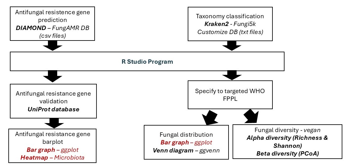
Fungal Metagenomics Data Pipeline Summary