Fungi functional guild (FunGuild) plot
This is a basic Fungi functional guild (FUNGuild) plot tutorial.This tutorial dose not require installation, you can simply use Rstudio Cloud on your browser.
เว็บเพจนี้สอนวิธีการวิเคราะห์ข้อมูล Fungi functional guild (FUNGuild) เบื้องต้น โดยผู้เรียนไม่ต้องดาวน์โหลดโปรแกรมลงบนคอมพิวเตอร์ส่วนตัว เพียงใช้ Rstudio Cloud
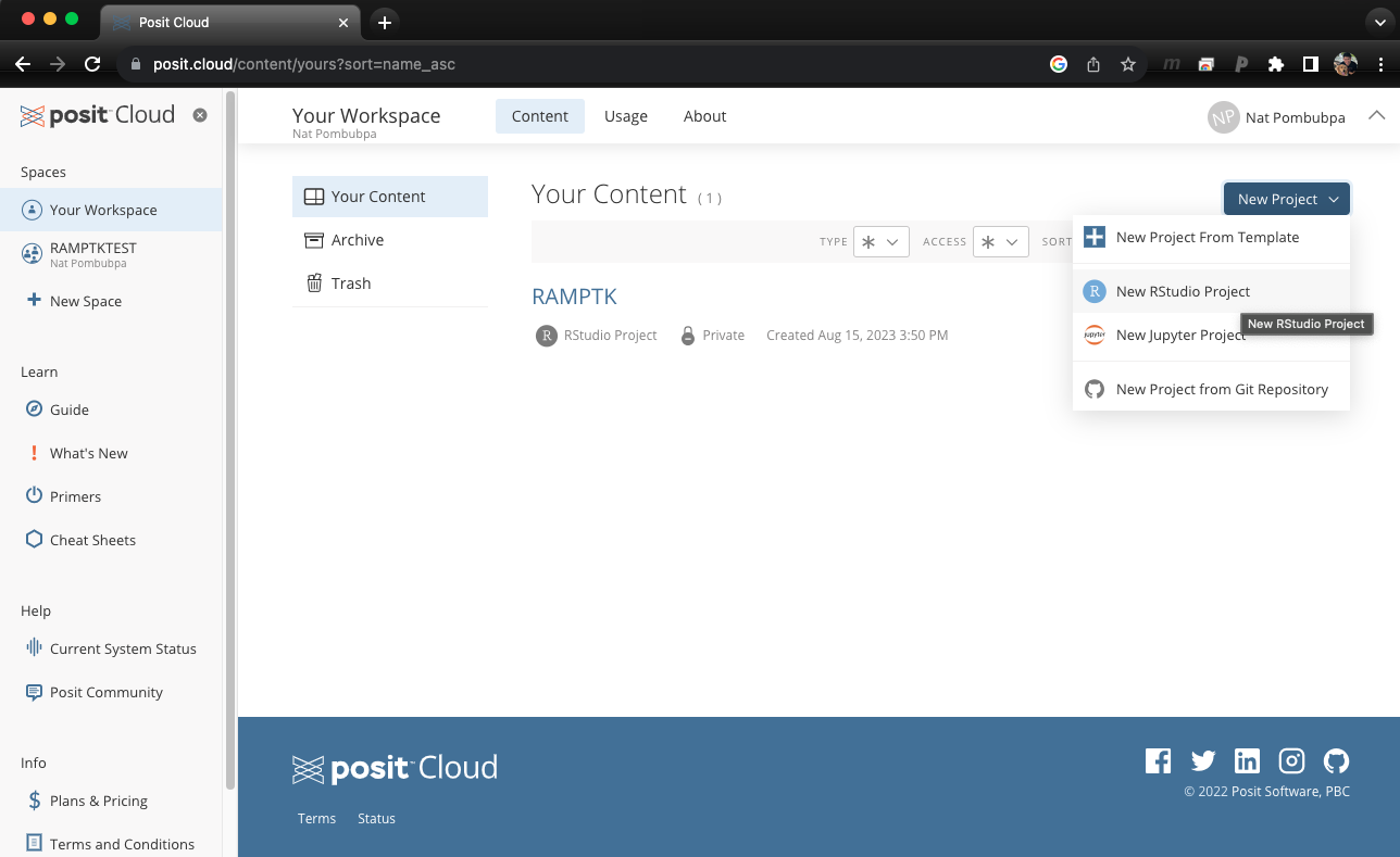
Step A: Open Rstudio cloud and Launch Console

Once you log in to Rstudio cloud, your web browser should bring up a similar window as the picture shown above. Click the button on the top right corner to create a new Rstudio project. Then, the next step is to click “Terminal” which should look like a picture below after you click on it.
Step 1: Downloding example data
FUNGuild: An open annotation tool for parsing fungal community datasets by ecological guild.
Once we identify fungal taxonomy/species, the next step that would be crucial for microbial ecology is to learn about fungal ecologyical functions. Our example data were generated using FUNGuild which annotate fungal function to each species in our dataset. Today, we will learn how to go from FUNGuild output to generating composition plot.
#Download FUNGuild example data
/cloud/project$ wget --no-check-certificate 'https://drive.google.com/uc?export=download&id=1rNnaGHxRp-qR78I0YaDwC02HBabLs-6I'

#Rename example data filename
/cloud/project$ mv uc\?export\=download\&id\=1rNnaGHxRp-qR78I0YaDwC02HBabLs-6I FUNGuild_example.txt
Step 2: Downloding example mapping file
Not only that we need FUNGuild data, we will also need to have mapping file which will have information about our samples.
#Download example mapping file
/cloud/project$ wget --no-check-certificate 'https://drive.google.com/uc?export=download&id=1xNUfmeD63t4j7E4MKTmJuoYwSsZNRRpU'

#Rename example mapping file filename
[/home/jovyan]$ mv uc\?export\=download\&id\=1xNUfmeD63t4j7E4MKTmJuoYwSsZNRRpU mapping_File.txt
Now, you should have mapping_File.txt and FUNGuild_example.txt in your folder
#Check your files
/cloud/project$ ls
FUNGuild_example.txt  mapping_File.txt
Step 3 : Preprocessing step
Oftentime, bioinformatic processes begin with preprocessing step or reformatiing your files. In this example, our sample name in mapping_File.txt and FUNGuild_example.txt do not match. Therefore, we will change sample names in FUNGuild_example.txt to match sample names in our mapping_File.txt.
Note: Don’t do these steps if your file samples name doesn’t use -: skip to step 4
#Check original sample names in FUNGuild_example.txt
/cloud/project$ head -1 FUNGuild_example.txt
#OTU ID GMT-CLC GMT-CLC-SUB     GMT-GLC GMT-GLC-SUB     TaxonomyTaxon    Taxon Level     Trophic Mode    Guild   Confidence Ranking

#Change sample names in file
/cloud/project$ sed '1s/-/\./g' FUNGuild_example.txt > FUNGuild_example_fix.txt

#Check new sample names in FUNGuild_example.txt
/cloud/project$ head -1 FUNGuild_example_fix.txt
#OTU ID GMT.CLC GMT.CLC.SUB     GMT.GLC GMT.GLC.SUB     TaxonomyTaxon    Taxon Level     Trophic Mode    Guild   Confidence Ranking    Growth Morphology       Trait   Notes   Citation/Source
We will use R to generate FUNGuild plot, but R will skip a line that begins with #. Our file header begin with #OTU, therefore, we will need to change to OTU.
#Change header of FUNGuild_example_fix.txt
/cloud/project$ sed '1s/#OTU/OTU/g' FUNGuild_example_fix.txt > FUNGuild_example_fix_header.txt
Step 4: Generating a plot in R
Open R by clicking on “Console”
First, install packages in R
install.packages("ape", "ggplot2")
install.packages("vegan")
install.packages("dplyr")
If run into this error Error: package or namespace load failed for ‘dplyr’ in loadNamespace(j <- i[[1L]], c(lib.loc, .libPaths()), versionCheck = vI[[j]]):
there is no package called ‘pillar’, you can fix it by
install.packages("pillar", dependencies = TRUE)
Then, try installing dplyr again.
if (!require("BiocManager", quietly = TRUE))
    install.packages("BiocManager")

BiocManager::install("phyloseq")
After installation is completed, we can begin the analysis.
First: check working directory
getwd()
If it’s not where your data located, you will need to setwd
setwd("/cloud/project/FUNGuild/")
Then, you can start the analysis.
#Code for Rscript
#Load R libraries
library(ape)
library(vegan)
library(dplyr)
library(phyloseq)
library(ggplot2)

#Load mapping file into R
meta <- read.table("mapping_File.txt",header=TRUE,row.names=1,sep="\t",stringsAsFactors=FALSE)
sampleData <- sample_data(meta)

#Load reformatted FUNGuild data into R
FG <- read.table("FUNGuild_example.txt",header=T,sep="\t",row.names=1)

#Select only the column that we need
FGotus <- select(FG, -(Taxonomy:Citation.Source))
FGotumat <- as(as.matrix(FGotus), "matrix")
FGOTU <- otu_table(FGotumat, taxa_are_rows = TRUE)
FGtaxmat <- select(FG, Confidence.Ranking, Trophic.Mode, Guild, Growth.Morphology)
FGtaxmat <- as(as.matrix(FGtaxmat),"matrix")
FGTAX = tax_table(FGtaxmat)

#Creating phyloseq object
physeq = phyloseq(FGOTU,FGTAX,sampleData)
physeq.prune = prune_taxa(taxa_sums(physeq) > 1, physeq)
physeq.prune.nopossible = subset_taxa(physeq.prune, Confidence.Ranking="Highly Possible")
physeq.prune.nopossible = subset_taxa(physeq.prune.nopossible, Confidence.Ranking!="-")

#Create color palette
cbbPalette <- c("#009E73","#999999", "#E69F00", "#56B4E9", "#F0E442", "#0072B2", "#D55E00", "#CC79A7", "midnightblue", "lightgreen","saddlebrown", "brown", "aquamarine4","lavenderblush2","snow3", "darkblue", "darkgoldenrod1", "darkseagreen", "darkorchid", "darkolivegreen1", "black","lightskyblue", "darkgreen", "deeppink", "khaki2", "firebrick", "brown1", "darkorange1", "cyan1", "royalblue4", "darksalmon", "darkblue","royalblue4", "dodgerblue3", "steelblue1", "lightskyblue", "darkseagreen", "darkgoldenrod1", "darkseagreen", "darkorchid", "darkolivegreen1", "brown1", "darkorange1", "cyan1", "darkgrey")

#Create a plot
FUNGuildcom = ggplot(data = psmelt(physeq.prune.nopossible), mapping = aes_string(x = "Sample" ,y = "Abundance", fill = "Trophic.Mode" )) + geom_bar(stat="identity", position="fill") + ggtitle("Fungal Trophic Mode Composition ")+theme(axis.text.x = element_text(angle = 90, hjust = 1)) + scale_fill_manual(values = cbbPalette)

#Take a look at our plot
FUNGuildcom
#Save a plot to PDF file
pdf("./Fungal Trophic Mode Composition.pdf", width = 8, height = 5)
FUNGuildcom
dev.off()
pdf
After the run is completed, you should see a PDF file in your current directory. Your result should be similar to the picture shown below.

Practice with bigger dataset
There are four example files that you can try.
- https://drive.google.com/uc?export=download&id=1Gme74xcEtzf4uWUsW85JcU_RHaZMHthk
- https://drive.google.com/uc?export=download&id=1SsenarC3xDhWiG24FX1JsWS7QZeL0KGi
- https://drive.google.com/uc?export=download&id=158oEC_-ULEfuck3gokTF-rP2KcnfJHYP